What the measurement actually means
Allan deviation examines how the variability of averaged measurements changes with averaging time. For inertial sensors it can help distinguish time scales dominated by different stochastic behaviors, but it is not a direct end to end navigation accuracy measurement. The result depends on record duration, stationary conditions, data handling, and the estimator used. A visually neat curve with a minimum is insufficient evidence for a specific error model, particularly when temperature drift or environmental changes are mixed into a supposedly stationary test.
A reproducible working procedure
Collect a long uninterrupted stationary record with known units and regular timestamps, preserving the sensor temperature. Check for missing samples, warmup transients, saturation, and changes in filtering before calculation. Use a documented overlapping or nonoverlapping Allan estimator and identify which one was chosen. Calculate each sensor axis separately. Restrict reported averaging times to those supported by enough independent information; the longest averaging windows often have weak statistical support. Keep the input record and analysis settings so another reviewer can reproduce the curve.
Illustrative calculation and interpretation
For an illustrative 3,600 second record sampled at 100 hertz, there are 360,000 samples. A ten second cluster contains 1,000 samples and provides many more comparisons than a 900 second cluster. Only four nonoverlapping 900 second blocks fit in the hour, so the long time estimate is inherently much less stable. This counting exercise does not prescribe a universal cutoff. It shows why plotting an attractive tail at very long averaging times cannot replace adequate duration or uncertainty assessment.
Quality checks and failure diagnosis
Compare repeated recordings rather than selecting the lowest observed minimum as the sensor specification. Inspect whether an apparent slope persists over a meaningful interval and whether the physical test conditions support that interpretation. Do not convert a curve parameter into guaranteed map accuracy by multiplying it by a flight duration. Navigation uses multiple sensors and constraints, and model errors can dominate. Use the analysis to justify a stochastic model or further testing, then validate that model through independent residual behavior and realistic operating trials.
Build an evidence chain
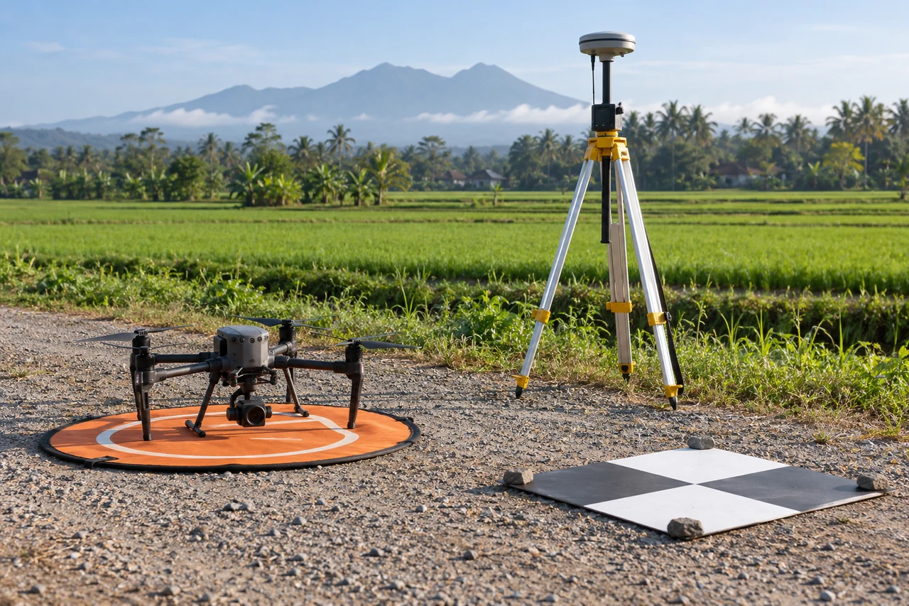
Keep the original receiver observations, camera event records, sensor configuration, and processing log together before editing anything. Work on copies and record file checksums so that a later discrepancy can be traced to a particular input. A useful evidence table links each image name to its event time, trajectory record, solution status, and exclusion reason. Missing entries deserve investigation before a reconstruction starts; an attractive map cannot restore observations that were never recorded or establish which clock supplied an undocumented timestamp.
Separate precision from reference accuracy
A tightly clustered navigation solution describes repeatability under the assumptions used by its estimator. It does not prove that the base coordinate, height system, sensor origin, or camera exposure time is correct. Treat those items as separate parts of the measurement chain. First inspect internal consistency, then compare against independent surveyed features that were withheld from any adjustment. Report a directional bias as well as scatter, because an almost constant displacement can coexist with a very small estimated position standard deviation.
Design a controlled comparison
Change one processing choice at a time and retain both outputs. Compare a common time interval and the same image subset, rather than allowing different exclusions to disguise the effect. Plot the coordinate differences against time, speed, turning rate, and solution status. A step, a smooth drift, and a periodic oscillation suggest different mechanisms. Write down the expected signature before looking at the result; this reduces the temptation to explain every pattern after the fact or to choose settings merely because their report looks better.
Make uncertainty operational
Create an uncertainty register with columns for source, units, possible bias, temporal behavior, and the evidence used to estimate it. Combine independent random components through variance only when independence is defensible. Keep shared reference errors and unknown systematic effects visible instead of dividing them by the number of photographs. Translate the resulting uncertainty into the actual task: locating an asset, comparing elevations, or estimating a boundary displacement may require different acceptance decisions even when they use the same underlying image collection.
Check independent locations
Distribute independent checks through the mapped footprint and across relevant surface types. Record how each reference point was measured, how its center was identified in the output, and whether the surrounding terrain permits a stable comparison. Inspect residual arrows and height differences spatially, then summarize the valid sample with its count and coverage. Do not silently delete difficult checks. Investigate them, document exclusions, and distinguish a demonstrated acquisition problem from a reference measurement or interpretation problem before accepting the deliverable.
Preserve the release context
The handover should state the observation date, coordinate reference frame, vertical convention, time scale, sensor offsets, processing version, and checks actually performed. Include any interval that relies on a degraded navigation solution and explain how those images were handled. Preserve a machine readable manifest beside a short human readable note. A reviewer should be able to reproduce the selection of usable observations and understand the limits without access to the original operator or a screenshot of a temporary application dashboard.
Test the decision, not just the file
Define the downstream decision before choosing an acceptance tolerance. An overview map, a repeat survey comparison, and an engineering measurement can use similar looking files while requiring different evidence. Write the tolerance in physical units and state the footprint where it applies. If the available checks do not cover a surface type or operating condition, identify that gap explicitly. This makes a conditional acceptance useful: the analyst can release a supported portion, retain a flagged portion for investigation, and avoid silently extending evidence beyond the locations actually examined.
Distinguish an assumption from an observation
Keep a short interpretation note separating measured quantities, calculations, and assumptions. The numerical example in this article is an illustration of a mechanism; replace its inputs with project measurements before making an operational decision. For an uncertain input, repeat the calculation over a defensible range and see whether the conclusion changes. If it does, obtaining better evidence for that input may be more valuable than adjusting unrelated processing settings. Retain the alternative results so a reviewer can understand why the selected workflow was judged adequate.
Using the result in a mapping project
Orthomosaic Mapping Software is most useful here when its outputs remain connected to the documented inputs and checks. A DroneCollab project can be considered as one processing destination, while the analyst retains responsibility for coordinate interpretation, independent validation, and suitability for the intended measurement. Confirm the available import and export options for the actual project rather than assuming that a product name establishes support or accuracy.