The site decision and observation unit
This guide examines zonal statistics denominators when a mapping team needs to build an interpretable city-feature inventory with stable identifiers. The goal is to connect a specific technical choice to observable site evidence, an independently checkable comparison and a clear delivery decision.
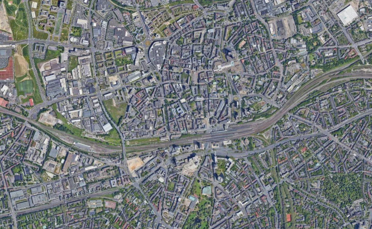
Define the object class before tracing: roof outlines, building footprints, road surfaces and parcel boundaries serve different purposes. Use stable identifiers and a documented interpretation scale. Dense urban blocks contain overlapping vertical surfaces, so a clean polygon is not necessarily the intended ground-level object. Record source date and observation limitations for each class.
Define the decision before choosing a processing configuration. State the target object, the observable surface, the required geographic reference and the evidence needed by the receiving user. Separate direct observations from inferred values. This prevents an attractive image from becoming an unsupported claim about conditions that the sensor did not observe. Preserve the project question in the run record so later quality review evaluates the intended use rather than a convenient software statistic.
The technical mechanism
Zonal statistics summarize raster information within defined polygons. The result depends on valid coverage, cell-inclusion rules and the meaning of the values. A mean, a class proportion and a total answer different questions. Small or irregular zones are sensitive to grid boundaries, so the denominator must be explicit before the table is interpreted.
Site conditions that can mislead interpretation
Tall buildings displace roofs, narrow streets are shadowed and courtyards may be hidden. Vehicles and temporary objects change between views. Legal boundaries cannot be inferred simply from visible fences or roofs. A geometrically valid dataset can still mix incompatible object definitions and produce misleading area totals.
A complete table can conceal incomplete raster support. A plausible average is not evidence that the whole management unit was observed.

Prepare the inputs and the controlled test
Validate polygon geometry and identifiers, then confirm raster and vector references. Define how partial cells and missing observations are handled. Manually check a small representative zone. Keep valid cell count or covered area alongside the statistic. For categorical data, preserve class meanings rather than averaging arbitrary numeric codes.
Build the comparison around a preserved baseline. Use the same input inventory, geographic extent and independent reference observations whenever the experiment permits. Change one justified factor at a time and record any unavoidable difference. Select both a difficult inspection region and a stable control region before examining the candidate output. Compare on their common valid support, then report any gain or loss of total coverage separately. This distinguishes a local improvement from a result that merely excludes the hardest observations.
Independent verification in this setting
Review a stratified sample including tall structures, low buildings, shadows and difficult boundaries. Check topology and compare uncertain interpretations with suitable independent evidence. Keep coordinate accuracy checks distinct from semantic validation. Resolve whether a disputed edge represents a roof, wall base or another feature before changing the geometry.
Compare results near zone boundaries and in partially observed units. Check whether overlapping zones intentionally count the same area more than once. Inspect the effect of grid alignment on small units. Retain the source raster and zone versions so the table can be reproduced.
A linked check: Raster Resampling Choices
Resampling estimates values on a different grid. Nearest-neighbor selection, interpolation and aggregation serve different data meanings. A method suitable for continuous elevation may be unsuitable for categorical classes. The target grid alignment and cell size influence which observations contribute, so a conversion must preserve both the geographic reference and the semantic meaning.
Identify whether values represent continuous measurements, class identifiers, counts or densities. Choose a documented method appropriate to that meaning. Test a small extract with recognizable boundaries and known values. Preserve the original raster, target grid definition and validity mask so changes can be traced to the resampling operation.
Compare selected values, class integrity and boundary behavior on common support. Review statistics using the correct units and denominator. Inspect for a half-cell displacement or unexpected smoothing. Confirm the receiving application reads the intended reference and numeric type.
An illustrative decision example
Consider an illustrative management polygon that overlaps several raster cells, with part of its area outside the valid observation mask. A summary computed only from valid cells can be useful, but it does not describe the entire polygon unless the missing portion is addressed appropriately. Report the coverage denominator with the statistic. If a later conversion changes the missing area to zero, the same polygon may acquire a different mean even though none of the observed values changed. Inspect selected cells, grid alignment and validity behavior through the actual export path. For a categorical raster, check class counts rather than averaging arbitrary class identifiers. This hypothetical comparison demonstrates why a successful file conversion and a plausible table are insufficient evidence of analytical equivalence. Preserve the source and receiving definitions so another analyst can explain whether a difference arose from a physical observation, a grid choice or a changed interpretation of missing data.
Interpret uncertainty before accepting the result
Write the acceptance rule before selecting the most attractive output. The actual threshold must follow the project purpose and the quality of the independent evidence. Inspect signed differences and spatial patterns as well as summaries. Investigate consequential outliers using their source observations instead of deleting them to improve a score. A result can be suitable for inspection planning while remaining unsuitable for a more demanding engineering or quantitative claim. State that intended-use boundary explicitly.
Deliver evidence that the next team can use
Deliver feature definitions, stable identifiers, confidence notes and topology rules. Preserve uncertain or unobservable objects instead of forcing a complete inventory. Receiving GIS users should know exactly what each polygon represents and which interpretation evidence supports it.
Keep the accepted source dates, processing version, coordinate conventions, masks and reference evidence beside the delivered data. Reopen a representative output from a clean copy and confirm that the intended receiving application interprets it consistently. Identify any remaining unsupported areas and the additional observation that would resolve them. The next analyst should be able to reconstruct the decision without depending on a temporary browser session, an operator recollection or a file whose name merely says final.
Where a cloud workflow can help
Online Photogrammetry Software can simplify the transfer from an organized image collection to a shared review workflow, but it does not remove acquisition or validation responsibilities. Drone Collab can be considered as part of that workflow after the team checks the current published capabilities and the outputs required by the project. Start with a representative collection and evaluate the evidence, usability and handover together. Choose the workflow because it supports a defensible decision rather than because one preview looks particularly polished.