The measurement question and its physical mechanism
Why can a tiny site be harder to map reliably than an open field many times its size? This is a practical question for teams evaluating Cloud Photogrammetry Software, because the usefulness of a mapping product depends on the observations and decisions that support it.
A small parcel can be dominated by buildings, trees, obstructions, and boundaries. Few straight flight segments may fit inside it, leaving turns, occlusion, and edge effects to occupy a large fraction of the available views.
A flight plan translates an information requirement into camera positions, exposure timing, and visible surface coverage. The useful plan is the one the recorded images can demonstrate, not merely the one drawn by the planning interface. Start with the feature that must be interpreted, identify the conditions most likely to remove its detail, and test those conditions in a representative short capture. Safety, permissions, and the limitations of the aircraft remain acquisition constraints even when a theoretically attractive geometry would improve reconstruction.
Acquisition and input preparation
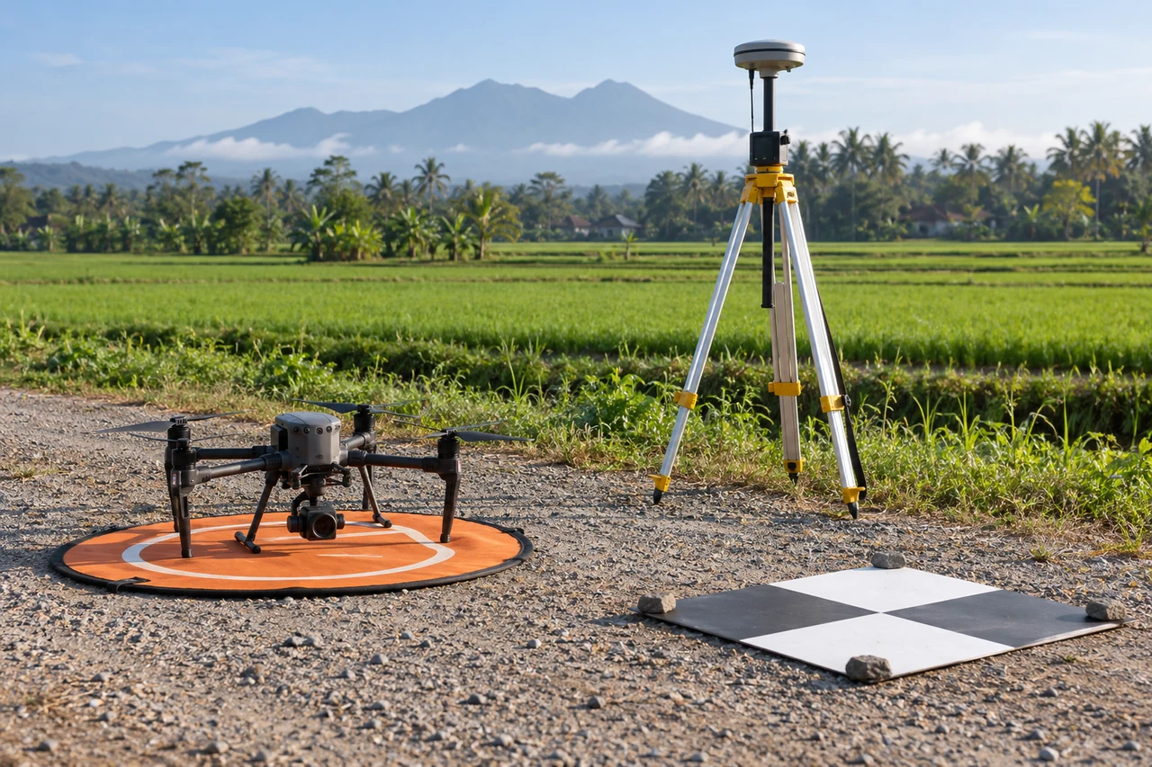
Plan safe and permitted coverage outside the parcel where possible, with a capture buffer and views that connect visible ground. Identify inaccessible corners before promising uniform coverage.
After acquisition, inspect the actual sequence rather than relying exclusively on nominal settings. Review sharpness, sustained triggering, changing ground distance, and the first and last useful views on each line. Compare those observations with the intended boundary and the surfaces the user needs. A local acquisition weakness often calls for a targeted supplementary view or revised capture window; increasing every processing setting consumes resources without necessarily changing the physical information available.
Illustrative worked example
The following numbers are hypothetical planning inputs, not measured product results or an accuracy claim. Suppose a parcel measures 60 m by 40 m and is surrounded by trees and buildings. A 10 m internal boundary band occupies 2,400 − 40 × 20 = 1,600 square meters, or two thirds of the parcel. This simple area example shows why edge behavior can dominate a small site. A large footprint over the parcel does not ensure the ground corners are visible from useful directions. Inventory each critical corner and distinguish visible ground from canopy or roof. Where an external capture buffer is safe and authorized, use it to bring the parcel into a stronger interior block. Otherwise document the unobservable regions and obtain complementary measurements rather than implying complete aerial ground coverage.
What the example means for this topic
Small parcels require visibility planning because boundary effects consume much of the site. Distinguish roofs and canopy from the ground that the user actually intends to measure. A complete-looking raster can hide those substitutions. Where external coverage is constrained, explain the observable limits and use complementary measurements for critical ground or boundary features that aerial views cannot establish.
A reproducible processing experiment
Inspect the parcel boundary independently of the broader reconstruction. Compare source visibility and image directions for each critical corner, and do not equate a complete surrounding map with a complete parcel survey.
Make the comparison reproducible before changing the workflow. Freeze a working copy of the image inventory and give the baseline a clear run identifier. Save the relevant camera configuration, image preparation steps, processing settings, requested outputs, and comparison extent. Select inspection regions that include the mechanism under investigation as well as a stable control region. A useful control is a surface expected to remain unaffected by the proposed change, because it can reveal whether an apparent local improvement introduces a broader adverse effect elsewhere in the block.
Change one justified factor at a time whenever practical. Use the same physical features and independent reference observations in the baseline and candidate. Compare on their common valid area, then report any difference in total supported coverage separately. Keep display zoom, color stretch, and viewing direction consistent when screenshots are part of the evidence. Record resource use and failures as outcomes too: a configuration that slightly improves detail but repeatedly exceeds available memory may not be operationally suitable for the agreed delivery.
Write the decision rule before examining the most attractive output. For example, the candidate may need to retain all critical features, reduce an identified systematic pattern, and avoid a new coverage gap. The actual thresholds must come from the project purpose and reference quality, not from the illustrative numbers in this article. Preserve both the accepted and rejected experiment records long enough to explain the choice. This is especially valuable when a later operator needs to repeat the workflow under different light, camera, or software conditions.
Diagnosing the result
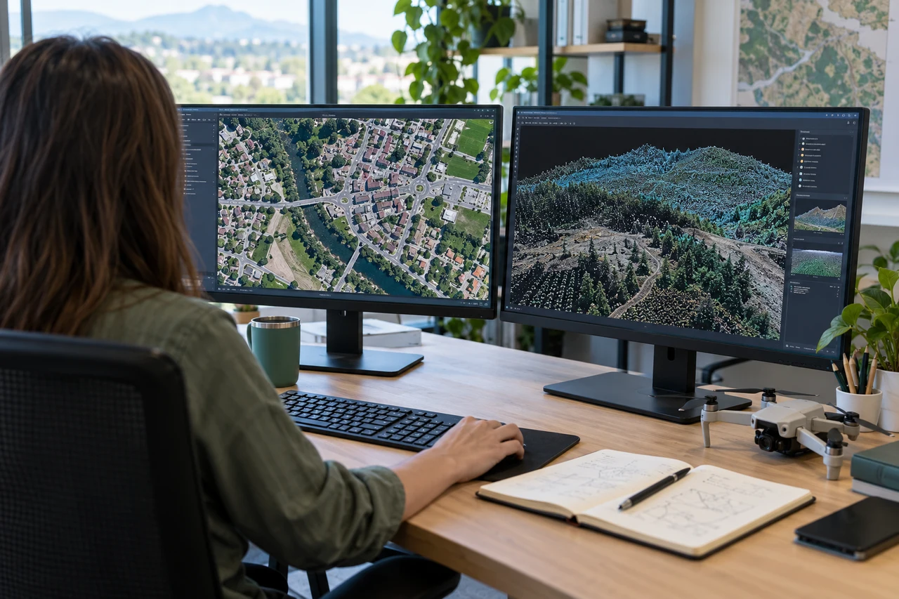
A colored patch inside the polygon may be a roof or canopy rather than ground. A small positional discrepancy can matter greatly when the parcel's features are close together.
Uncertainty and independent quality checks
Separate internal agreement from independent product validation. Observations used to fit camera positions, calibration, or a surface cannot by themselves establish external accuracy. Reserve suitable checks when the measurement task requires them and document the uncertainty of those checks. The reference should identify the same physical feature that appears in the map or model; a precise survey of an ambiguous edge can still produce an uncertain comparison. Inspect signed differences and spatial patterns, because a single average can hide a broad bias or one consequential local failure.
Keep uncertainty statements tied to the quantity being used. Horizontal location, height, distance, surface completeness, and visual interpretability are not interchangeable. Pixel spacing is a sampling property, and point density is a representation property; neither alone specifies the error of a derived measurement. Do not convert a camera-model residual directly into a universal ground-accuracy claim. If evidence is limited to a pilot region or one surface class, state that scope and avoid extending the conclusion to untested materials, distant boundaries, or hidden surfaces.
Unknown areas should remain identifiable. A smooth mesh, filled raster, balanced image, or sharp texture can be useful for communication while containing information inferred from its surroundings. Retain masks or an edit record for consequential inferred regions, and choose additional observations when the missing evidence affects the decision. Where a formal specification applies, use its required sampling and reporting procedure rather than treating this explanatory workflow as certification. The practical goal is a defensible statement about supported use, with enough evidence for another team to assess its limits.
The practical decision and delivery record
Deliver the physical surfaces actually observed, qualify occluded corners, and use complementary measurements when the intended boundary or ground feature cannot be established from aerial imagery.
The accepted handoff should contain a concise inventory of the authoritative outputs and the evidence needed to interpret them. Include the acquisition interval, surface definitions, relevant units and reference information, coverage boundary, input manifest, accepted configuration, and material quality findings. Open the downloaded files in an appropriate independent reader and inspect difficult regions as well as easy ones. Preserve an unambiguous version identifier so a recipient does not accidentally measure an earlier experimental export that happens to have a similar filename.
Translate each remaining limitation into a practical consequence. State which feature, area, or use it affects and whether the appropriate next step is another view, a complementary measurement, a different representation, or a narrower interpretation. Avoid a generic high-quality label when one critical region remains unsupported. A short explanation attached to the relevant location is more useful than an impressive global statistic that leaves users to discover the exception after making a consequential decision.
Testing a suitable cloud workflow
Teams comparing Cloud Photogrammetry Software can include DroneCollab in a representative pilot workflow. Its mapping outputs include orthomosaics, point clouds, DSM/DTM products, and textured three-dimensional models, with GNSS/PPK workflows available for relevant projects. Choose the output that answers the physical question, then inspect the exported evidence using the checks described here. Product availability does not establish a particular survey accuracy, and a successful processing job still needs project-specific review before its results support measurements or operational decisions.